This post is the third part of a tutorial on t-SNE. The first part introduces dimensionality reduction and presents the main ideas of t-SNE. The second part introduces the notion of perplexity. The present post covers the details of the nonlinear embedding.

On the origins of t-SNE

If you are following the field of artificial intelligence, the name Geoffrey Hinton should sound familiar. As it turns out, the “Godfather of Deep Learning” is the author of both t-SNE and its ancestor SNE. This explains why t-SNE has a strong flavor of neural networks. If you already know gradient-descent and variational learning, then you should feel at home. Otherwise no worries: we will keep it relatively simple and we will take the time to explain what happens under the hood.

We have seen previously that t-SNE aims to preserve a relationship between the points, and that this relationship can be thought of as the probability of hopping from one point to the other in a random walk. The focus of this post is to explain what t-SNE does to preserve this relationship in a space of lower dimension.

The Kullback-Leibler...

In this tutorial, I would like to explain the basic ideas behind t-distributed Stochastic Neighbor Embedding, better known as t-SNE. There are tons of excellent material out there explaining how t-SNE works. Here, I would like to focus on why it works and what makes t-SNE special among data visualization techniques.

If you are not comfortable with formulas, you should still be able to understand this post, which is intended to be a gentle introduction to t-SNE. The next post will peek under the hood and delve into the mathematics and the technical detail.

Dimensionality reduction

One thing we all agree on is that we each have a unique personality. And yet it seems that five character traits are sufficient to sketch the psychological portrait of almost everyone. Surely, such portraits are incomplete, but they capture the most important features to describe someone.

The so-called five factor model is a prime example of dimensionality reduction. It represents diverse and complex data with a handful of numbers. The reduced personality model can be used to compare different individuals, give a quick description of someone, find compatible personalities, predict possible behaviors etc. In many...

The code is written in a very naive style, so you should not use it as a reference for good C code. Once again, the purpose is to highlight the mechanisms of the algorithm, disregarding all other considerations. That said, the code runs so it may be used as a skeleton for your own projects.

The code is available for download as a Github gist. As in the second part, I recommend playing with the variables, and debugging it with gdb to see what happens step by step.

Constructing the suffix array

First you should get familiar with the first two parts of the tutorial in order to follow the logic of the code below. The file learn_bwt_indexing_compression.c does the same thing as in the second part. The input, the output and the logical flow are the same, but the file is different in many details.

We start with the definition of the occ_t...

It makes little sense to implement a Burrows-Wheeler index in a high level language such as Python or JavaScript because we need tight control of the basic data structures. This is why I chose C. The purpose of this post is not to show how Burrows-Wheeler indexes should be implemented, but to help the reader understand how it works in practice. I tried to make the code as clear as possible, without regard for optimization. It is only a plain, vanilla, implementation.

The code runs, but I doubt that it can be used for anything else than demonstrations. First, it is very naive and hard to scale up. Second, it does not use any compression nor down-sampling, which are the mainsprings of Burrows-Wheeler indexes.

The code is available for download as a Github gist. It is interesting for beginners to play with...

There are many resources explaining how the Burrows-Wheeler transform works, but so far I have not found anything explaining what makes it so awesome for indexing and why it is so widely used for short read mapping. I figured I would write such a tutorial for those who are not afraid of the detail.

The problem

Say we have a sequencing run with over 100 million reads. After processing, the reads are between 20 and 25 nucleotide long. We would like to know if these sequences are in the human genome, and if so where.

The first idea would be to use grep to find out. On my computer, looking for a 20-mer such as ACGTGTGACGTGATCTGAGC takes about 10 seconds. Nice, but querying 100 million sequences would take more than 30 years. Not using any search index, grep needs to scan the whole human genome, and this takes time...

A couple of months ago, I posted an approximate formula for the longest match in the problem of DNA alignment. I recently used it to calibrate a seeding heuristic to map Illumina reads and I was surprised to see that it was not just bad, but epic bad. Upon closer inspection, I realized that the main assumption does not hold when the error rate is small (which is typically the case for Illumina reads). The formula was based on longest runs in Bernoulli trials. This time I present more accurate results with an approach based on a stick breaking process.

Stick breaking (spacings)

Inserting $(k)$ mutations at random in a sequencing read will produce $(k+1)$ (possibly empty) subsequences without errors. The process is analogous to inserting $(k)$ breaks at random in a stick of length 1, and we can approximate the distribution of the longest subsequence without error by that of the longest fragment when breaking the stick.

The example above illustrates this concept graphically. A sequencing read of 60 nucleotides contains 2 mutations highlighted in red and the longest error-free stretch is the central subsequence of 28 nucleotides. If mutations occur uniformly on the read...

A brief note published a few weeks ago initiated a discussion on the blogosphere about who is a bioinformatician and who is not. According to Wikipedia

bioinformatics combines computer science, statistics, mathematics, and engineering to study and process biological data.

To see how the community defines itself, I downloaded the abstracts of Bioinformatics from 2014 (for a total around 1000 articles, extracted the most relevant keywords and put the top 100 terms in a word cloud where a word size shows its frequency^*.

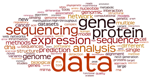
Obviously, bioinformatics is about data, mostly gene/protein sequences and expression. It is also good to know that bioinformatics likes genomes and networks, and that it has more affinities with structural biology than with evolution.

The favourite organism of bioinformaticians is Homo sapiens, actually it is the only one mentioned in the word cloud, and when bioinformaticians work on a disease, it is cancer.

When bioinformaticians describe their work, it is “novel” and “new”, and what they talk about is “biological”, “different”, “multiple” and “single” (the last two are usually followed by “sequence alignment” and “nucleotide polymorphism”). It is also “functional” and “available”, but somewhat less. I expected it to be “fast” and “accurate”, but...

I never planned to do bioinformatics. It just happened because I liked to spend time in front of my computer and my boss was OK with it. Still, as every sane individual, I sometimes think that I should do something else with my life, and I wonder whether I am doing the right thing. On this topic, I recently came across the famous farewell to bioinformatics by Frederick J. Ross, which is worth reading, and from which the most emblematic quote is the now celebrated aphorism

Fuck you, bioinformatics. Eat shit and die.

There is nothing to agree or disagree in this quote, but Frederick gives further detail about his point of view in the post. In short, bioinformaticians are bad programmers, and community-level obfuscation maintains the illusion.

By making the tools unusable, by inventing file format after file format, by seeking out the most brittle techniques and the slowest languages, by not publishing their algorithms and making their results impossible to replicate, the field managed to reduce its productivity by at least 90%, probably closer to 99%.

There are indeed many issues in the bioinformatics community and I am on Frederick’s side regarding file formats...

1. Cars would have nice names

Here is what an abstract describing a car would look like.

Transporting people to defined locations of interest is a challenge of significant economic importance. To achieve this goal, people usually use cars or public transport. However, these solutions are suboptimal in several conditions. For instance, when people are extremely close to their target location, both cars and public transport are inappropriate, which limits their practical use. Here we present CaЯ (vehiCle for chAnging geo-cooЯdinates), a fast and accurate tool as an alternative to existing vehicles.

2. Cars would be fast and accurate

Bioinformaticians develop fast and accurate software. Their cars would be just the same. Here is what a typical benchmark sections would look like.

To show that CaЯ is faster and more accurate than existing alternatives, we benchmarked CaЯ against Volvo XC90 and Ferrari F430. In the first series of tests, we measured the time to lower the front windows of the vehicles. The average run duration was 2.3 seconds for CaЯ, 3.1 seconds for Volvo XC90 and 3.9 seconds for Ferrari F430, which demonstrates that CaЯ is substantially faster than Volvo XC90 and Ferrari...

The problem of sequence alignment gets a lot of attention from bioinformaticians (the list of alignment software counts more than 200 entries). Yet, the statistical aspect of the problem is often neglected. In the post Once upon a BLAST, David Lipman explained that the breakthrough of BLAST was not a new algorithm, but the careful calibration of a heuristic by a sound statistical framework.

Inspired by this idea, I wanted to work out the probability of identifying best hits in the problem of long read alignments. Since this is a fairly general result and that it may be useful for many similar applications, I post it here for reference.

Longest runs of 1s

I start with generalities on...