In this post I explain what perplexity is and how it is used to parametrize t-SNE. This post is the second part of a tutorial on t-SNE. The first part introduces dimensionality reduction and presents the main ideas of t-SNE. This is where you should start if you are not already familiar with t-SNE.

What is perplexity?

Before you read on, pick a number at random between 1 and 10 and ask yourself whether I can guess it. It looks like my chances are 1 in 10 so you may think “no there is no way”. In fact, there is a 28% chance that you chose the number 7, so my chances of guessing are higher than you may have thought initially. In this situation, the random variable is somewhat predictable but not completely. How could we quantify that?

To answer the questions, let us count the possible samples from this distribution. We ask $(N)$ people to choose a number at random between 1 and 10 and we record their answers $((x_1, x_2, \ldots, x_N))$. The number 1 shows up with probability $(p_1 = 0.034)$ so the total in the sample is approximately $(n_1 = p_1 N)$. The same holds for $(n_2, \ldots, n_{10})$ that are computed from $(p_2, \ldots, p_{10})$. Now, the number of ways to form a sample of size $(N)$ where the number 1 appears $(n_1)$ times, the number 2 appears $(n_2)$ times etc. is given by the multinomial coefficient $$\frac{N!}{n_1! n_2!\ldots n_{10}!}.$$ We can use the Stirling formula $(x! \sim x^x e^{-x}\sqrt{2\pi x} )$ to simplify the number above as $$2^{NH+O(\log N)} \text{ where } H = p_1 \log_2 \frac{1}{p_1} + \ldots + p_{10} \log_2 \frac{1}{p_{10}}.$$

The term $(H)$ is known as the binary entropy of the distribution, and we just showed that the number of samples of size $(N)$ from a distribution with entropy $(H)$ is approximately $(2^{NH})$. In plain English, the entropy of a distribution measures how fast the combinatorics explode when you draw samples from this distribution.

It is thus natural to consider the rate of exponential increase $(2^{H})$. It can be thought of as the number of samples of size 1, or more intuitively the effective size of the random set (the size of a uniform random set with the same entropy). This term is called the perplexity and it is just an alternative way of measuring the entropy.

Back to our example, the entropy of the human random choice is approximately 3.053 bits, and the perplexity is approximately 8.30. Even if 10 options are available, humans behave as if they were choosing from only 8 (actually just a little higher). This is of course an approximation, but it gives the main idea of what perplexity stands for and how to interpret it. This also shows how it can be used to quantify how predictable a random variable is.

Perplexity in t-SNE

It is important for t-SNE that each point gets approximately the same number of neighbors, otherwise the projection will come out wrong. For instance, imagine a dense set of points lying on a sphere in high dimension, plus one single point at the center. If the sphere is large, the point at the center has no neighbor. In the projected space, the points on the sphere will form a compact mass, but the point at the center is not their neighbor so it will be projected far away. Ideally, we would like this point to remain at the center after the projection, but for this, it must be the neighbor of the points on the sphere.

Perplexity comes in handy because it allows us to define a nominal number of neighbors for every point. Remember from the previous post that t-SNE defines neighborhoods from hopping probabilities. If we force the hopping probabilities from every point to have the same perplexity, say 30, we are in effect making hops equivalent to choosing one of 30 neighbors at random.

Mathematically, the hopping probability from point $(i)$ to point $(j)$ is defined using Gaussian weights as

$$p_{j|i}(\sigma_i) = \frac{\exp \big(-|x_i-x_j|^2 \big/ 2\sigma_i^2 \big)}{\sum_{j \neq i}\exp \big(-|x_i-x_j|^2 \big/ 2\sigma_i^2 \big)},$$ where $(x_i)$ and $(x_j)$ are the coordinates of points $(i)$ and $(j)$ before the projection, and $(\sigma_i)$ is a free parameter. The entropy of the of hopping probabilities from point $(i)$ to any of the $(N)$ points of the data set is

$$H(\sigma_i) = p_{1|i} \log \frac{1}{p_{1|i}} + \ldots + p_{N|i} \log \frac{1}{p_{N|i}}.$$

For a target perplexity $(\eta)$, we are thus looking for $(\sigma_i)$ such that $(2^{H(\sigma_i)} = \eta)$, or equivalently $(H(\sigma_i) = \log_2 \eta)$.

$(H(\sigma_i))$ does not simplify further, so finding $(\sigma_i)$ must be done numerically. Fortunately, this is not very difficult. When $(\sigma_i)$ increases, the Gaussian weights are more similar to each other so the hopping probabilities become uniform and the entropy tends to its maximum (among all the distributions over $(N)$ points, the uniform is the one with the highest entropy). So there can be only one $(\sigma_i)$ that solves the equation, and it is straightforward to use bisection to find it.

In pictures, this is relatively simple. Suppose that the full space is a plane, as in the sketch below.

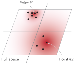
When a point $(i)$ is in a dense region (like point #1), the value of $(\sigma_i)$ is small so that the Gaussian weights are non negligible in a small circle around point $(i)$. Conversely, if point $(i)$ is in a sparse region (like point #2), the value of $(\sigma_i)$ is large and the circle around the point is large. In the sketch above, the intensity of the red pixels represents the relative values of the Gaussian weights. The spread is wider for point #2 than for point #1.

How does perplexity impact the projection?

The perplexity parameter of t-SNE is usually presented as a tuning knob to balance the representation of local versus global features in the projection. With the above interpretation in mind, we see why this is the case. At low perplexity, every point has few neighbors (only the few closest points), and only those small neighborhoods will be preserved after the projection. This typically results in disconnected neighborhoods of size approximately equal to the perplexity, that are projected as small clusters on the t-SNE plane.

Conversely, when perplexity is high, each point has a large neighborhood and its location after projection depends on points that were originally far away. This tends to generate large connected clusters on the t-SNE plane.

At the extreme, when perplexity is larger than the number of points, the equation above has no solution for $(\sigma_i)$ because the maximum perplexity of a distribution over $(N)$ points is $(N)$. What happens next depends on the t-SNE implementation, but this is mostly uninteresting because it does not depend on the data set any more.

Let us see this with an example. Consider the data points below. They consist of two separate Gaussian clusters of 100 points in a 3D space.

Below are projections of this data on a t-SNE plane at different values of perplexity. At perplexity 5 and 10, the gray and red clusters are broken up into smaller clusters of size approximately 5 and 10. At perplexity 100 the clusters have their original appearance. Also note that the red point that accidentally came closer to the gray cluster is projected to the same location at the periphery of the gray cluster, facing the red cluster.

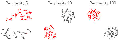
This example shows that at low perplexity, the small-scale features are emphasized, at the expense of the large-scale features, like the gray and red clusters, which are distorted. At high perplexity this is the reverse.

Conclusion

Perplexity has an intuitive interpretation if we think of it as the size of an equivalent random set. For t-SNE, the perplexity parameter corresponds to the approximate size of the smallest neighborhoods after projection. This is what allows the user to highlight small-scale or large-scale clusters in the data.

Further reading

The posts below contain a lot of additional information about how to understand and tune perplexity in t-SNE.

1. How to Use t-SNE Effectively
2. How to tune hyperparameters of tSNE