This post is the third part of a tutorial on t-SNE. The first part introduces dimensionality reduction and presents the main ideas of t-SNE. The second part introduces the notion of perplexity. The present post covers the details of the nonlinear embedding.

On the origins of t-SNE

If you are following the field of artificial intelligence, the name Geoffrey Hinton should sound familiar. As it turns out, the “Godfather of Deep Learning” is the author of both t-SNE and its ancestor SNE. This explains why t-SNE has a strong flavor of neural networks. If you already know gradient-descent and variational learning, then you should feel at home. Otherwise no worries: we will keep it relatively simple and we will take the time to explain what happens under the hood.

We have seen previously that t-SNE aims to preserve a relationship between the points, and that this relationship can be thought of as the probability of hopping from one point to the other in a random walk. The focus of this post is to explain what t-SNE does to preserve this relationship in a space of lower dimension.

The Kullback-Leibler divergence

In general, relationships between points cannot remain exactly the same in lower dimension. All we can hope for is to not distort them too much, so we need some measure of similarity. Since we express the neighborhood relationship as a probability, we can use the Kullback-Leibler divergence to compare the neighborhoods before and after projection.

The Kullback-Leibler divergence is a measure of dissimilarity between two probability distributions. We can use it to find a replacement distribution that is most similar to a target distribution, just like in variational learning. In other words, given a target distribution $(Q)$ and a search space $(S)$, we are interested in $$ {\arg\min}_{P \in S} \text{ KL}(P||Q).$$

In the present context, the Kullback-Leibler divergence is used only as a pseudo-distance. If you would like to learn more about it, you can refer to this post about the use of the Kullback-Leibler in statistics. But here, all we need to know is that given $(P)$ and $(Q)$ two distributions over the events $(a_1, \ldots, a_N)$, the Kullback-Leibler is by definition $$\text{KL}(P||Q) = -\sum_{i=1}^N \log \frac{Q(a_i)}{P(a_i)}P(a_i).$$

In t-SNE, the target distributions $(Q)$ are the hopping probabilities in the original space, and the approximations $(P)$ are the hopping probabilities after the projection. To give a concrete example, consider the hopping probabilities in the sketch below.

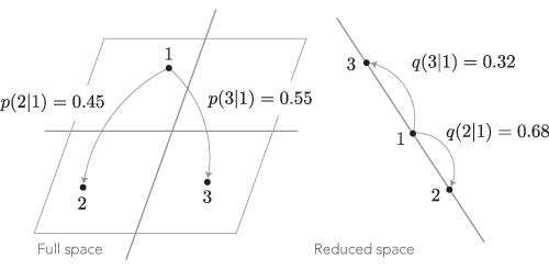
Using the Kullback-Leibler divergence as a dissimilarity measure for the hopping probabilities from point 1, we obtain $$KL_{(1)} = -0.45\log\frac{0.68}{0.45} -0.55\log\frac{0.32}{0.55} \approx 0.112.$$

This gives us a measure of how much the hopping probabilities from point 1 have changed, but to get a complete picture, we also need to take into account the hopping probabilities from every other point, as we are about to see.

The probability distributions

There are not one but many probability distributions. Indeed, for each point $(i)$, we can hop to any other point $(j)$, so there is a different distributions $(Q(cdot|i))$ for every data point $(i)$. One of the main improvements of t-SNE over SNE is that it replaces this collection of distributions by a single symmetric probability distribution over the pairs of points: $$Q^*(j,i) = Q^*(i,j) = \frac{Q(j|i) + Q(i|j)}{2N},$$

where $(N)$ is the number of points in the data set. As we will see below, this trick makes it relatively easy to find a good projection, or more precisely to find a minimum of the Kullback-Leibler divergence. Note that in the random walk interpretation, $(Q^*(i,j))$ is not the probability of observing a hop from $(i)$ to $(j)$ or from $(j)$ to $(i)$. It is only a probability over the pairs of points with a convenient symmetry.

We have seen in the first part of this series that the hopping probabilities are based on Gaussian weights. Concretely, they are defined for every pair of points $(i \neq j)$ as $$Q(j|i) = \frac{\exp \big(-||x_i-x_j||^2 \big/ 2\sigma_i^2\big)}{\sum_{k \neq i} \exp \big(-||x_i-x_k||^2 \big/ 2\sigma_i^2\big)}.$$

The terms $(Q(\cdot|i))$ define a probability distribution where $(Q(i|i) = 0)$. The quantity $(\sigma_i)$ is a free parameter (actually, those are $(N)$ parameters) and its value is set so that the perplexity of the distributions $(Q(\cdot|i))$ are all equal to some chosen target (see the second part). The terms $(Q^*(\cdot|\cdot))$ define a symmetric probability distribution over the pairs $((i,j))$.

In parallel, t-SNE must define a single symmetric distribution over the pairs of points after the projection. In t-SNE it is based on weights inspired from the Student's t distribution with one degree of freedom, also known as a Cauchy distribution. More specifically, $$P(j|i) = \frac{\big(1 + ||y_i - y_j||^2\big)^{-1}}{\sum_{k \neq i} \big(1 + ||y_i - y_k||^2\big)^{-1}}.$$

The terms $(P(\cdot|i))$ also define a probability distribution where $(P(i|i) = 0)$, this time without free parameter. We again need a symmetric distribution over the pairs $((i,j))$, and since $(P(\cdot|\cdot))$ is already symmetric, we can take $(P^*(j|i) = P(j|i)/N)$.

The distribution $(Q^*(\cdot|\cdot))$ is completely determined as soon as the perplexity parameter is chosen. The distribution $(P^*(\cdot|\cdot))$ is determined by the positions $(y_i)$ of the projected points. We thus need to find the positions $(y_i)$ that minimize $$\text{KL}(P^*||Q^*) = -\sum_{i \neq j} \log \frac{Q^*(j|i)}{P^*(j|i)}P^*(j|i).$$

The projection problem has now been turned into an optimization problem with $(pN)$ variables, where $(p)$ is the dimension of the embedding (usually 2) and $(N)$ is the number of points in the data set.

Gradient descent

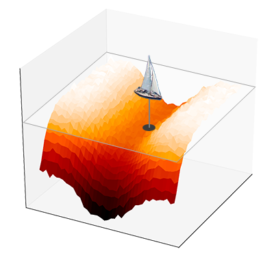
Modern learning algorithms are mostly based on the concept of gradient descent. This is an optimization algorithm inspired from physics, where a ball rolls downhill until it reaches a low point and its speed vanishes. Likewise, the idea of gradient descent is to feed some random initial values to a function and change them so as to decrease the value of the function until we hit a minimum.

The analogy with the rolling ball is misleading because we can see the landscape and we always know where the ball will go next. A better analogy by David McKay is that of a boat trying to locate the lowest point of the ocean by probing the bedrock. The probe must also measure the slope of the oceanic floor in order to decide where to go next. In other words, the gradient of the function to optimize is the key to finding the minimum — I personally prefer to think of gradient descent as the way we search the source of a smell or a sound, because it is easier to imagine what this means in higher dimensions.

A limitation of gradient descent is that it can stall dramatically at saddle points. One can think of saddle points as valleys, with a near-horizontal slope even though the function is not close to a local minimum. This is not really an issue for modern optimizers, but t-SNE is based on the standard version of gradient descent, so it does tend to stall.

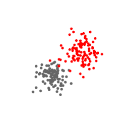
The points above represent a three-dimensional dataset. Their t-SNE projection in two dimensions is shown below, at every iteration of the algorithm. Notice how the points stop moving for a while before expanding and taking a shape that is a good approximation of the original data.

Here we can tell when the algorithm is stuck and when it has converged, but in higher dimension, there is no way to differentiate one from the other. Therefore, it is recommended to have too many rounds of t-SNE optimization rather than too few. Either way, it is one of the main limitations that one cannot really tell whether the algorithm is trapped in a saddle point.

Back to the optimization problem, it turns out that computing the gradient is fairly simple. The point of using the Cauchy distribution and symmetric distributions over the pairs $(Q^*(\cdot|\cdot))$ and $(P^*(\cdot|\cdot))$ is precisely to simplify the gradient. If you would like to know more about this, the original article gives a very detailed derivation of the gradient in the appendix.

The process runs how you may expect: you start from a random configuration and at every iteration you compute the gradient and move the points by a small step along that gradient. After several iterations the points stop moving because you found an optimum and the gradient goes to zero. Your projection is ready!

Epilogue

This concludes a relatively deep introduction to t-SNE. The method is slowly being replaced by UMAP, which enjoys some significant advantages (especially in terms of speed). Still, it is very useful to understand the concepts behind t-SNE because they are based on the fundamental aspects of machine learning that made neural networks what they are today.

There is a lot of material out there about t-SNE. I particularly recommend this blog post and the posts of Nikolay Oskolkov on Medium, particularly this one and that one.