There are many resources explaining how the Burrows-Wheeler transform works, but so far I have not found anything explaining what makes it so awesome for indexing and why it is so widely used for short read mapping. I figured I would write such a tutorial for those who are not afraid of the detail.

The problem

Say we have a sequencing run with over 100 million reads. After processing, the reads are between 20 and 25 nucleotide long. We would like to know if these sequences are in the human genome, and if so where.

The first idea would be to use grep to find out. On my computer, looking for a 20-mer such as ACGTGTGACGTGATCTGAGC takes about 10 seconds. Nice, but querying 100 million sequences would take more than 30 years. Not using any search index, grep needs to scan the whole human genome, and this takes time when the file is large.

We could build an index to speed up the search. The simplest would be a dictionary that associates each 20 to 25-mer to its locations in the human genome. The nice thing about dictionaries is that the access time is fast and does not depend on the size of the text.

The issue is space. Counting 2 bits per nucleotide, 20 to 25-mers take 40 to 50 bits of storage. The human genome contains over 3.2 billion nucleotides, so we need at least 108 GB (in reality many 20 to 25-mers are repeated so this number would be lower). To this we should add the storage required for the locations and the overhead for the dictionary, for a total size well over 200 GB.

So it seems that we are between a rock and a hard place: either we run out of time, or we run out of memory.

The suffix array

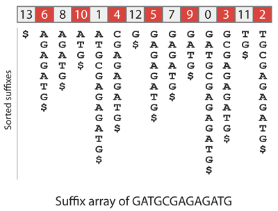
An important step towards modern algorithms was the invention of a data structure called the suffix array of a text. A suffix is the end of a text from a given position. For instance, the 1st suffix of GATGCGAGAGATG is GATGCGAGAGATG itself, and the 10th is GATG (I will use the 0-based convention, so 1st, 2nd, 3rd etc. refer to positions 0, 1, 2 etc.). The suffix array stores the positions of the suffixes sorted in alphabetical order.

Let us construct the suffix array of GATGCGAGAGATG for demonstration. We add a terminator character $, which has lower lexical order than all other characters (this avoids confusion when comparing strings of different lengths). As a consequence, the first suffix in lexical order is always $. Below are the suffixes in sorted order (written vertically) and the suffix array of GATGCGAGAGATG.

How can we use the suffix array of the human genome to solve the query problem above? Since the suffixes are sorted, we can proceed by bisection. We lookup the middle entry of the suffix array, which points to a particular position of the human genome. We compare the query to the sequence at that position, and depending on the result we continue bisecting either on the left half or on the right half of the suffix array.

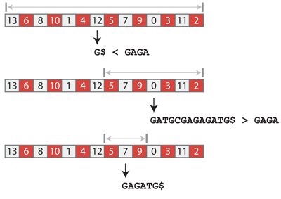
Let us use this technique to find how many occurrences of GAGA are in GATGCGAGAGATG. The suffix array has 14 entries, so we look up the entry at position 6 (remember the 0-based convention), which points to the suffix G$. Since GAGA > G$, we continue bisecting in the positions of the suffix array between 7 and 13 included. The middle entry is at position 10 and points to the suffix GATGCGAGAGATG$. Since GAGA < GATGCGAGAGATG$, we continue bisecting between positions 7 and 9 included. The middle entry is at position 8 and points to the suffix GAGATG$. This time we have a hit because GAGATG$ starts with GAGA. By continuing the bisection, we would find that suffixes at position 7 and 8 start with GAGA, so the query is present two times in the text.

Why is this an improvement? The suffix array of the human genome has $(N)$ = 3.2 billion entries, so we need at most $(\lfloor\log_2(N)\rfloor +1 = 32)$ steps to find out whether any query is present or not. We would need a few extra steps to find out the number of occurrences in case it is present. Each step consists of 2 memory accesses, one in the suffix array, one in the human genome to read the suffix. Counting approximately 100 ns per memory access and ignoring the time for string comparison, this brings us around 6-7 us per query. Now what about the space requirements? We can encode every position of the genome with a 4 byte integer, and we need to store 3.2 billion entries, so we need 11.92 GB. Still a lot, but notice that this approach solves all the practical difficulties associated with dictionaries. We can easily look for sequences of any length in the suffix array.

The Burrows-Wheeler transform

The Burrows-Wheeler transform of a text is a permutation of this text. To construct it, we need to sort all the suffixes, but we replace the whole suffix by the preceding letter. For the suffix equal to the text itself, we write the terminator $ instead. The previous sketch shows that the Burrows-Wheeler transform of GATGCGAGAGATG is GGGGGGTCAA$TAA, as can be verified below.

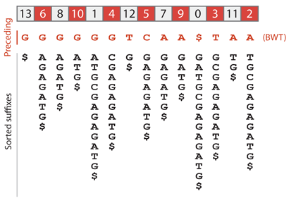
Before explaining how this will help, let us highlight a fundamental property of the Burrows-Wheeler transformed text. Note that in the sketch above, the nucleotides appear in sorted order in the row immediately below the Burrows-Wheeler transform. See that the first G in the Burrows-Wheeler transformed text is the one preceding $. It is also the first G to appear in the sorted text. The second G in the Burrows-Wheeler transformed text is the one preceding AGAGATG$. It is also the second G in the sorted text. The first T in the Burrows-Wheeler transformed text is the one preceding G$. It is also the first T in the sorted text. More generally, the letters of the Burrows-Wheeler transformed text are in the same “relative” order as in the sorted text.

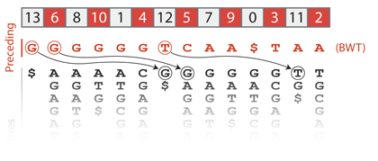
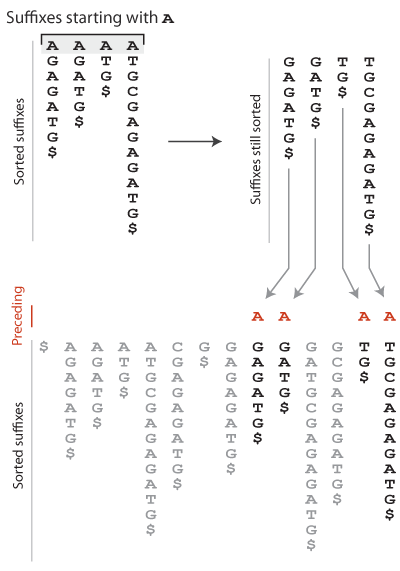
This is called the “First-Last property” of the Burrows-Wheeler transform. The sketch below helps understand why it holds. Let us consider the suffixes in sorted order, and more particularly those that start with A. If we remove this A, we obtain another series of suffixes. The key point is that they are still in sorted order because the A was not discriminant. These suffixes are somewhere in the set of all sorted suffixes. There can be some other suffixes between them, but their relative order does not change because they were already sorted. Now, these suffixes are preceded by A so their positions are the positions of A in the Burrows-Wheeler transformed text. Looking at the whole process, it is clear that the relative order of A in the sorted text is the relative order of A in the Burrows-Wheeler transformed text. Of course, the same holds for every character.

The First-Last property is the key to using the Burrows-Wheeler transformed text for search. The next section will explain how this is done.

The backward search

Let us illustrate how the Burrows-Wheeler transformed text can be used to look for GAGA in the text. All the occurrences of GAGA in the text end with A. Each A is also the first letter of some suffix of the text. Because such suffixes all start with A, they are stored next to each other in the suffix array, namely between positions 1 and 4. However, only those suffixes preceded by a G can potentially contain the query. This is exactly the information encoded by the Burrows-Wheeler transformed text. In this concrete example, all the As are preceded by a G, so the text contains 4 suffixes that start with GA.

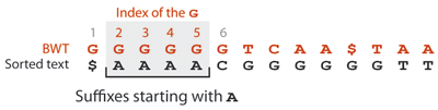
Since those 4 suffixes start the same way, they are stored next to each other in the suffix array, but where? The Gs preceding the As are the 2nd, 3rd, 4th and 5th Gs in the order of the Burrow-Wheeler transformed text, so they are also the 2nd, 3rd, 4th and 5th Gs in the sorted text. Knowing that the position of the first G is 6, the suffixes that start with GA are thus stored in positions 7 to 10 of the suffix array.

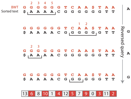
The process continues as we read the query backwards. The target suffixes must be preceded by an A. According to the Burrows-Wheeler transformed text, two suffixes are preceded by an A, and since their relative order is the same as in the sorted text, we know that the suffixes starting with AGA are at positions 1 and 2 of the suffix array. Finally, to complete the suffix GAGA, the target suffixes must be preceded by a G. According to the Burrows-Wheeler transformed text, both suffixes at positions 1 and 2 are preceded by G and, again, since their relative order is the same as in the sorted text, we know that the suffixes starting with GAGA are at positions 7 and 8 of the suffix array.

The Occ table

Real world implementations of the backward search are based on a data structure called the Occ table (Occ stands for occurrence). The table contains the cumulative number of occurrences of each character in the Burrows-Wheeler transformed text. It also comes together with an array called C that stores the position of the first occurrence of each character in the sorted text.

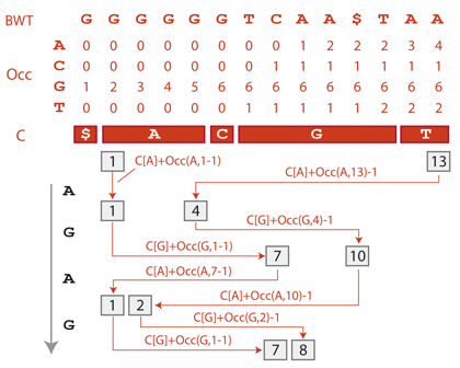
With these data structures, the backward search of GAGA goes as follows: Before we start, suffixes can be at any position of the suffix array between 1 and 13 (position 0 always corresponds to the prefix $). The first suffix starting with A is stored in the suffix array at positions C[A] = 1 (by definition). The number of suffixes starting with A is equal to the number of As in the text, i.e. to Occ(A,13) = 4. So the suffixes starting with A are stored between positions 1 and 4 of the suffix array.

How many of those suffixes are preceded by a G?. The number of Gs appearing in the Burrows-Wheeler transformed text before position 1 is Occ(G,1-1) = 1, and the number appearing up until position 4 is Occ(G,4) = 5, so the number of Gs preceding the suffixes between positions 1 and 4 is 5-1 = 4. There are thus 4 suffixes starting with GA. One G occurs before them (i.e. Occ(G,1-1) = 1), so they are the 2nd till 5th Gs in the Burrows-Wheeler transformed text, and also in the suffix array. Since the first suffix starting with G is stored at position C[G] = 6 of the suffix array, the 2nd till 5th suffixes are stored between positions 7 and 10.

These boundaries can obtained directly as C[G] + Occ(G,1-1) = 6+1 = 7 and C[G] + Occ(G,4)-1 = 6+5-1 = 10. To continue the process, we find the positions of the suffixes starting with AGA between positions C[A] + Occ(A,7-1) = 1+0 = 1 and C[A] + Occ(A,10)-1 = 1+2-1=2. Finally, we find the positions of the suffixes starting with GAGA between positions C[G] + Occ(G,1-1) = 6+1 = 7 and C[G] + Occ(G,2)-1 = 6+3-1 = 8.

How does this algorithm perform? For a query sequence of length $(k)$, there are at most $(k)$ steps to perform, each with two memory accesses (the queries to Occ) for a total of $(2k)$ memory accesses. This number is independent of the size of the text, which is an extraordinary achievement.

What about the memory requirements? The Occ table contains one row per character of the alphabet and one column per character in the text, for a total of $(\sigma N)$ entries, where $(N)$ is the size of the text and $(\sigma)$ is the size of the alphabet. Each entry must be able to encode a number potentially as high as $(N)$, which requires $(\lfloor\log_2(N)\rfloor+1)$ bits, so the total size of the Occ table is $(\sigma N (\lfloor\log_2(N)\rfloor + 1))$ bits. For the human genome without reverse complement, this represents 47.68 GB. Considering that we also need the 11.92 GB suffix array, the benefits of the backward search seem doubtful. But the next section will change the deal.

Compression

What is truly awesome about Burrows-Wheeler indexing is that the search can be performed on compressed indexes. I will illustrate the simplest of many available options, in which the Occ table and the suffix array are merely down-sampled^*.

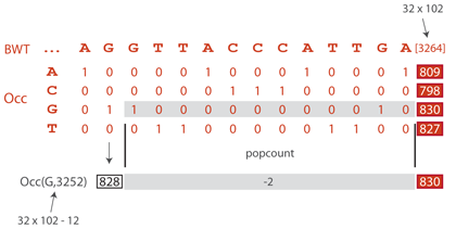
The Occ table stores the cumulative frequencies of the characters in the Burrows-Wheeler transformed text. If, instead, we stored their actual occurrence with a 0/1 encoding, we could still perform the backward search by counting the 1s until the given position of the text. To down-sample Occ, we keep one column out of 32 and we use the binary table to compute the missing values on demand. The picture above illustrates how Occ(G, 3252) is computed in a down-sampled table. The smallest multiple of 32 after 3252 is 3264. Looking up Occ(G, 3264), we find 830. We still need to remove the Gs between positions 3253 and 3264, which we do by counting the 1s in the binary table between these positions (this is called the popcount operation). The result is 2, so Occ(G, 3275) = 830-2 = 828.

The size of the binary table is $(\sigma N)$ bits. For the human genome, it represents 4 times 3.2 billion = 12.8 billion bits or 1.49 GB, so the total size of the Occ table is 1.49 + 47.68/32 = 2.98 GB. It is possible to store the down-sampled values of the Occ table together with the next 32 values of the binary table in a 64 bit word, so that a single memory access is necessary for each query to the Occ table. The popcount can be computed faster than a memory access (which is usually a last level cache miss here), so the backward search runs a little slower, but with a memory footprint 16 times smaller (2.98 GB instead of 47.68 GB).

We also compress the suffix array by keeping one value out of 32. The task is now to compute the missing values on demand. To show how this is done, let us illustrate a fundamental connection between the Burrows-Wheeler transformed text, the suffix array and the Occ table using once again the text GATGCGAGAGATG.

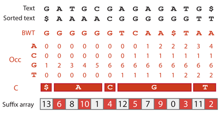
The suffix $ is stored at position 0 of the suffix array and contains the value 13. The Burrows-Wheeler transformed text at position 0 is G. Notice that C[G]+Occ(G,0)-1 = 6+1-1 = 6, which is the position of the suffix array that stores 12. At this new position, the Burrows-Wheeler transformed text is T. Notice that C[T]+Occ(T,6)-1 = 12+1-1 = 12, which is the position of the suffix array that stores 11. At this new position, the Burrows-Wheeler transformed text is A. Notice that C[A]+Occ(A,12)-1 = 1+3-1 = 3, which is the position of the suffix array that stores 10. More generally, if $(y)$ is stored at position $(m)$ of the suffix array, $(y-1)$ is stored at position C[X] + Occ(X,$(m)$)-1, where X is the value of the Burrows-Wheeler transformed text at position $(m)$.

This property allows us to use the Burrows-Wheeler transformed text and the Occ table to find out where the previous suffix is stored in the suffix array. To compute a value of the suffix array on demand, we just have to iterate this procedure, computing the position of the previous suffix at each step until this position is a multiple of 32. At that position the value of the suffix array is known. If it is equal to $(y)$ and $(k)$ iterations of the search were performed, then the position of the query in the text is $(y+k)$.

Each step of this procedure takes two memory accesses: one in the Burrows-Wheeler transformed text and one in the Occ table. Since we need 16 attempts on average to find a position that is a multiple of 32, we need on average 32 memory accesses to compute the values of the suffix array.

For the human genome, the size of the 32-fold down-sampled suffix array is 373 MB and that of the Burrows-Wheeler transformed text is 745 MB (assuming that we need two bits per character). The total size of our index is 2.98 GB + 373 MB + 745 MB = 4.07 GB. Obviously, it is possible to further down-sample the Occ table and the suffix array, at the cost of increasing memory accesses. Compressing the binary representation of the Occ table is also possible, but it requires more advanced knowledge of succinct data structures. With the index above, counting the occurrences of a query of length $(k)$ requires at most $(2k)$ memory accesses and knowing the position of each of them requires 64 memory accesses. For a unique 25-mer, this is about a hundred memory accesses or approximately 10 us (typically half in practice, because of cache effects). With this method, we can process millions of queries for an acceptable memory footprint.

Epilogue

The most natural application of Burrows-Wheeler indexing is to perform the seeding step of the DNA alignment problem. For instance, the popular mapper BWA uses the compression methods presented above. It is interesting to note that direct bisection on the suffix array has become a competitive algorithm as computers gained memory (the STAR mapper takes this approach). It costs only 64 memory accesses to find all the occurrences of a query in the human genome, vs that many per occurrence in the algorithm with compressed indexes. The weakness of the bisection method is that it still takes 64 accesses to know that a sequence is absent vs about 32 with compressed indexes (depending on the genome).

It is also worth mentioning that the Burrows-Wheeler transform is exceptionally well adapted to indexing the human genome. It gives simple algorithms for sub-string queries, and compressing the Occ table is most efficient on small alphabets. For proteins or natural languages, one would use indexes adapted to bigger alphabet, such as wavelet trees, or word-based indexes.

Further reading

There are many good texts explaining the mechanisms of the Burrows-Wheeler transform. I recommend the excellent textbook Bioinformatics Algorithms by Pavel Pevzner and Phillip Compeau, from which the demonstration of the First-to-Last property is inspired.