The story of this post begins a few weeks ago when I received a surprising email. I have never read a scientific article giving a credible account of a research process. Only the successful hypotheses and the successful experiments are mentioned in the text — a small minority — and the painful intellectual labor behind discoveries is omitted altogether. Time is precious, and who wants to read endless failure stories? Point well taken. But this unspoken academic pact has sealed what I call the curse of research. In simple words, the curse is that by putting all the emphasis on the results, researchers become blind to the research process because they never discuss it. How to carry out good research? How to discover things? These are the questions that nobody raises (well, almost nobody).

Where did I leave off? Oh, yes... in my mailbox lies an email from David Lipman. For those who don’t know him, David Lipman is the director of the NCBI (the bio-informatics spearhead of the NIH), of which PubMed and GenBank are the most famous children. Incidentally, David is also the creator of BLAST. After a brief exchange on the topic of my previous post, he gave me a detailed description of how he thought about BLAST with his team and what was on their mind at the moment they put the pieces of the puzzle together. Every bash against the curse of research is good to give, this is why I want to share this here. Yet, following this story may require some background on the state of affairs at the end of the 1980’s. Feel free to skip this update if you are familiar with sequence alignment.

Needleman-Wunsch

Modern sequence alignment started with Richard Bellman and dynamic programming. For a long time, I was puzzled by the “dynamic” part of dynamic programming. I finally found solace in this quote by Bellman himself admitting that it was a masquerade to protect his work from budget cuts.

[Dynamic] also has a very interesting property as an adjective, and that is its impossible to use the word dynamic in a pejorative sense.

This is my way of saying that I will not dwell on explaining what is dynamic programming because I myself find it very confusing. Instead, while I think of renaming this blog “The Grand Dynamic”, I will describe the standard application to the problem of aligning two sequences, which is known as the Needleman-Wunsch algorithm.

The key of the algorithm is to represent an alignment by a path in a matrix, as illustrated by the figure below. The two sequences to align are written at the top and left margins of the matrix. Starting from the top left corner, a path is drawn to the bottom right corner. A horizontal move consumes one character from the first sequence, a vertical move consumes one character from the second sequence, and a diagonal move consumes one character from both. The path shown in the example below represents one of the 8,989 ways to align YEKPCA with EKPCWA.

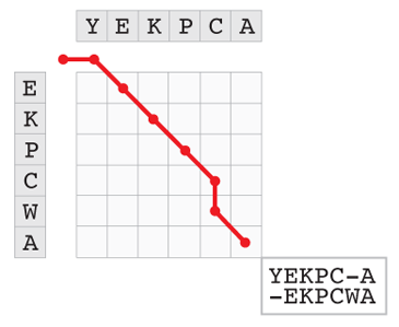
We can define a simple score to measure the quality of an alignment as the number of matches minus the number of mismatches (including insertions and deletions). It then makes sense to speak of the “best” alignment. However, the number of alignments explodes for long sequences, so that it becomes impossible to find the best alignment by systematic enumeration (if you are interested in the detail of how to compute the exact number of alignments, click on the Penrose triangle at the end of this section). The contribution of Needleman and Wunsch was to demonstrate that you do not need to explore all the paths to find the optimum. There is another way, and this one is immensely faster because it requires only a tiny fraction of this computational work.

The picture above is the fundamental property of exact sequence alignments. There are 3 ways to reach the bottom right corner of the matrix, representing 3 ways to finish the alignment between two sequences. Say that we are aligning sequences $(x)$ with $(y)$, and that $(x')$ and $(y')$ are the respective sequences where the last character is deleted. The picture shows that every alignment of $(x)$ with $(y)$ contains an alignment of either $(x')$ with $(y')$, or $(x)$ with $(y')$, or $(x')$ with $(y)$. If we knew the optimal scores corresponding to these 3 cases, we could know the optimal score for $(x)$ and $(y)$. All we would have to do is compute the 3 possible values of the scores after the last move and pick the highest.

We can apply the same rationale to the 3 cases recursively, which gives the optimal score by induction. All that remains to be done is initialize the algorithm. For this, we observe that the alignment score of the empty string and a sequence of length $(k)$ is $(-k)$ (for $(k \geq 0)$). We fill the margins of the alignment matrix and use the induction to fill it line by line with the optimal alignment scores between the substrings. The number in the bottom right cell is the best alignment score.

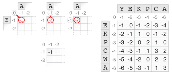
The picture above illustrates this process for YEKPCA and EKPCWA. The sketch on the left shows how the top left cell of the matrix is filled. A path through this cell can come from the diagonal, from the left, or from the top. In the first case, one letter is consumed from each string, and since they don’t match the score is -1. In the other two cases, only one letter is consumed, corresponding to a deletion in the other string which decreases the score by 1 for a final score of -2. The highest score out of these 3 cases is -1, which is written in the cell. The process is repeated for every cell to obtain the matrix shown on the right. The score of the optimal alignment is in the bottom-right cell, in this case it is 3, which corresponds to the alignment path shown in the first figure.

Smith-Waterman

What if we want to answer a slightly different question? Say we are not interested in the best alignment between two sequences per se, rather we want to know the best substring match between them. This is a fair question, since proteins typically contain functional domains arranged in families. Long stretches of homology may correspond to similar functions performed by similar protein structures.

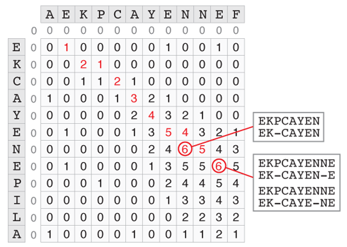
The Smith-Waterman algorithm, which is a variation of the Needleman-Wunsch algorithm tackles precisely this question. The major difference is that the smallest score that can be assigned to a cell at every step is 0. The cell with the highest score corresponds to the end of the best substring alignment. From there we can backtrack to the beginning of the match by following the path that led to this score. The example below shows how to find the best substring match between AEKPCAYENNEF and AECAYENEPILA. Two cells have a score of 6, but in the case of the second there are 2 possible backtraces. The 5 shown in red can either come from the 6 left of it by a horizontal move (insertion or deletion), or from the 4 at the top left by a diagonal move (match). So there are 3 optimal substring alignments with a score of 6.

Why does this work? If we follow the score along the best alignment path, a stretch of homology corresponds to an increase of the alignment score. In the Needleman-Wunsch algorithm, this burst towards higher values may start from a large negative alignment score and thus never reach a high level. In contrast, in the Smith-Waterman algorithm the burst always starts from a score of 0 or higher, so the amplitude of the biggest burst always corresponds to the highest score. To illustrate this idea, the image below shows the progression of the score along the same alignment for the two algorithms.

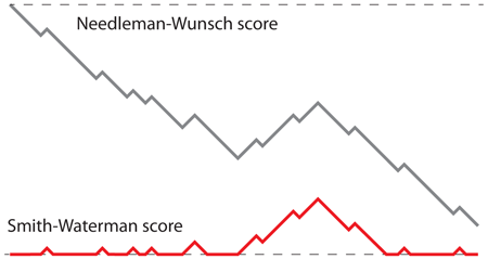
This picture is not only important to understand the difference between the algorithms, it also shows the connection between random walks and sequence alignment, which turned out to the be the cornerstone of BLAST.

Scoring matrices

Today, the field of sequence alignment thrives on genomics because high throughput DNA sequencing technologies generate a wealth of data that need to be analyzed. But at the time computer sciences were born, DNA could not be sequenced at all. Proteins on the other hand could be sequenced from the 1950’s by Edman degradation, so it is important to bear in mind that the alignment problem was initially driven by protein sequences.

The evolution of proteins is very different from the evolution of DNA. The 20 amino acids do not occur with similar frequencies in protein sequences, and replacement between amino acids with similar chemical properties (such as aspartic acid and glutamic acid) is a common phenomenon. For the purpose of detecting homology, aligned rare amino acids should have a higher contribution to the alignment score than common amino acids. Likewise, mismatches corresponding to replacements common in evolution should not penalize the alignment score.

These ideas were formalized by Margaret Dayhoff with the concept of Point Accepted Mutation matrices (PAM for short). PAM matrices have one row and one column per amino acid, and each entry gives the score of aligning a pair of amino acids. This scoring scheme combines harmoniously with the dynamic programming algorithms described above; the formalism is not changed when scores vary by fractional units. There is a lot to tell about scoring matrices, but for the sake of concision I have chosen to keep it to the minimum. What matters is that these adjustments are necessary, but they make the problem of understanding the statistical distribution of the score substantially more complex.

Seed-based methods

Even if dynamic programming is much faster than systematic enumeration, it is still not fast enough. Aligning two proteins of 1000 residues each means filling 1 million cells. Counting 1 microsecond per cell, this represents 1 second per alignment. Even for a tiny database of a thousand sequences, the queries are of the order of the hour, which is a no go for a public server.

The idea of David Lipman (among others) was to shortcut the sequence comparison by using heuristic methods, i.e. algorithms that do not guarantee to return the best alignment. The program FASTA (originally called FASTP), famous after the file format that bears its name, was an early implementation of this principle. The gist of FASTA is to look for perfect short matches between so called words of a given length and start the time-consuming but exact Smith-Waterman algorithm from those “seeds”.

Is this fast? Yes if the implementation is efficient. Suppose that all the words of length $(k)$ from the database have been indexed, i.e. the places they occur are stored in a lookup table that can be queried very fast. A cluster of word matches in the same region of a sequence hints that there may be a hit nearby, which is searched by the Smith-Waterman algorithm. In many cases, only a few subsequences of the database are selected after the first filter, which reduces the complexity of the problem and explains why it is fast. The exact detail of this procedure is given in reference [1].

Why does this sometimes fail? Because there is no guarantee that the best alignment is seeded, i.e. that it contains a perfect match for a word of length $(k)$. For instance, no homology would be detected between the two sequences shown below for $(k \geq 4)$ because their optimal alignment does not contain any match between words of length 4 or greater.

As David Lipman and William Pearson wrote FASTA, they realized the need to quantify the confidence in the hits. What are the chances that the best alignment has no match for words of length $(k)$, like the one shown above? This is a difficult question, and no solution was available at the time.

BLAST

It would take five more years and the talent of Samuel Karlin to solve this theoretical problem. The key insight, which turned out to be a very profound idea, was to treat the alignment between two unrelated proteins as a random walk. In the following excerpt from my correspondence with David Lipman, he explains how this happened.

I’d met Sam in the mid-80’s and recognized that he was in a different class from the statisticians and mathematicians involved in molecular biology. [...] I thought that locally optimal segments without gaps (i.e. using scoring matrices like PAM whose expected score was negative) might be more amenable to analysis yet still be useful for detecting subtle evolutionary relationships. Further, that this could possibly be extended to multiple alignments as well.

I visited Sam at Stanford and tried to convince him to work on the problem – he wasn’t interested initially but I insisted that this would be broadly useful so he agreed. It was within a matter of a few weeks, he got back to me indicating that they had essentially worked out the answer.

At that point, it took just a little push to assemble the pieces of the puzzle. Here is how the story continues.

One day while doing the dishes it sort of occurred to me that what Karlin’s results would allow you to do was to put the seed-based heuristic methods on a sound statistical framework [...]. That way you could use a rapid heuristic but estimate with confidence your chances of missing something. The BLAST idea of generating all short kmers with score of $(\geq s)$ came quite quickly and the basic algorithm was set. Initially I’d been thinking of pre-indexing the database but Webb Miller – who’d agreed to program this up – pointed out that for the similarity levels we were searching for, pre-indexing wouldn’t be efficient. Within a week of explaining the idea he’d sent me a program which performed well. Stephen joined us to work out the application of Karlin’s statistical approach to the matches, Gene worked on efficient gapped extensions (we didn’t have good statistics for those at the time so that wasn’t part of the original program), and Warren Gish proposed a [Finite State Machine] for more efficiently finding the word matches.

The people that David Lipman mentions are the authors of the original BLAST paper: Stephen Altschul, Warren Gish, Webb Miller and Gene Myers (see reference [2]).

BLAST proceeds in three phases. First, a list of high scoring words is extracted from the query. Those words are then compiled into a Deterministic Finite Automaton used to scan the database (like a regular expression). Finally, the dynamic programming alignments are computed from the seeds.

The first step requires some attention because it is one of the main differences with FASTA. Recall that for proteins, word matches of length $(k)$ can have different scores. BLAST ignores word matches below a certain score in order to keep only the best seeds for the subsequent alignment. To this end, all the words of length $(k)$ are extracted from the query, and the words scoring above a certain threshold when aligned to any of those words are collected. Those are the words used for seeding (typically, there are more such words than words of the query). Seeding with the words from the query is less efficient because it amounts to searching exact identity between the query and the database. The BLAST scheme searches high scoring matches, even if words are not identical between the query and the database.

The question that arises is what word length $(k)$ and what threshold to choose. As David Lipman mentions above, this is where Karlin’s result came in handy. For fixed word length and threshold, the probability that an alignment of score $(S)$ is not seeded (missed) decreases exponentially with $(S)$. Estimating the rate of decrease thus gives the chances of missing a hit of score $(S)$. For the required level of sensitivity, you can then choose the parameters maximizing the speed of the heuristic.

BLAST uses the limiting distribution of alignment scores provided by Karlin on two occasions. The first is to control the speed/precision balance of the heuristic. The second is to give the statistical significance of the hits. Many sources mention the second application, yet few mention how Karlin’s work was instrumental to tune the sensitivity of the heuristic.

Since then, BLAST has known an unprecedented success, it has spawned a whole family of software and entire books are dedicated to them. Yet, behind this success there is no algorithmic breakthrough. Instead, it is a unique combination of statistics and algorithms.

Epilogue

In a preliminary version of this post, I referred to Karlin’s work on sequence alignment as his major achievement. In spite of the scope of his result, this may not even be true, for he was very productive in several areas of mathematics. To clarify this, I will conclude with a final quote from David Lipman, and with my gratitude to him for his help in the writing of this post.

Sam had many incredibly important foundational contributions in statistics in addition to his books on stochastic processes (along with Howard Taylor) and on methods & theory in games & economics which have been immensely useful for many researchers.

References

[1] Rapid and sensitive protein similarity searches. Lipman and Pearson, Science. 1985 Mar 22;227(4693):1435-41.
[2] Basic local alignment search tool. Altschul, Gish, Miller, Myers and Lipman, J Mol Biol. 1990 Oct 5;215(3):403-10.