In July 1982, paleontologist Steven Jay Gould was diagnosed with cancer. Facing a median prognosis of only 8 months survival, he used his knowledge of statistics to prepare for the future. As he explains in The Median Isn’t the Message, if half of the patients died of this rare case of mesothelioma within 8 months, those who did not had much better survival. Evaluating his own chances of being in the “survivor” group as high, he planned for long term survival and opted out of the standard treatment. He died 20 years later, from an unrelated disease.

If not the median, then what is the message? Statistics put a disproportionate emphasis on the typical or average behavior, when what matters is sometimes in the extremes. This general blindness to the extremes is responsible for a dreadful lot of confusion in the bio-medical field. One of my all time favorite traps is the extreme value fallacy. Nothing better than an example will explain what it is about.

June babies and anorexia

If the perfect mistake was ever made, it definitely was in an article about anorexia published in 2001. A more accessible version of the story was published in the New Scientist, together with a few comments from the authors. Based on the observation that 51 out of 446 Scottish women suffering from anorexia are born in June, the article claims that “June babies have higher risk of anorexia”. There are two possible reactions to this statement. The first is to speculate why June babies are more fragile. The second is to wonder whether 51 out of 446 is a lot. Since the authors of the article do a pretty good job at the first, I will try to do an equally good job at the second.

We need a way to count how often 51 or more babies out of 446 are born in June, assuming that birth dates are random. For this purpose I wrote a simple R script to draw 446 birth dates randomly 10,000 times. Feel free to skip the code snippet if you don’t speak R, the results will speak for themselves.

# The function 'new_babies()' generates a random sample
# of size 12 containing the number of babies born each
# month. The argument 'size' is the total number of
# babies to distribute among the months. Illustrative
# function (not optimized for speed).
new_babies <- function(size) {
   # Trick to produce short month names.
   months <- format(ISOdate(2014,1:12,1), "%b")
   ndays <- c(31,28,31,30,31,30,31,31,30,31,30,31)
   x <- sample(months, size, prob=ndays, replace=TRUE)
   return(table(x))
}
# Function call with an example of output.
new_babies(446)
# Apr Aug Dec Feb Jan Jul Jun Mar May Nov Oct Sep 
#  45  35  40  30  35  47  38  30  36  35  33  42 

In the code below, I compute two numbers. The first is the number of babies born in June. The second is the largest number of babies born in any month of the year. This will tell me how often 51 or more babies are born in “some month”.

# You can reproduce this random example at home.
set.seed(123)
anorexia_June <- replicate(10000, new_babies(446)["Jun"])
anorexia_max <- replicate(10000, max(new_babies(446)))
mean(anorexia_June >= 51) # 0.0095
mean(anorexia_max >= 51)  # 0.1709

After running the simulation 10,000 times, we find that the chances that 51 or more babies are born in June are close to 1%. So 51 babies appears unusually high compared to the expected 36.66, which explains the conclusion of the authors. But the chances that a month of the year enumerates 51 or more babies are above 17%. In other words, it is fairly common that so many children are born in the same month.

The authors measure the second quantity — the maximum number of babies — but use the distribution of the first quantity — the number of babies in June. This seems justified because the maximum number of babies happens to be in June, but this is exactly what the extreme value fallacy is. June was never part of the hypothesis, it came ad hoc as a result of the measurement. Let’s use the result of the simulation again to demonstrate that the distributions of these two quantities are fundamentally different.

mean(anorexia_June) # 36.6635
mean(anorexia_max)  # 47.5374

In the simulation, the mean number of babies born in June is 36.6, fairly close to the expected value, but the maximum number of babies per month is at a much larger 47.54. Picking the maximum a posteriori, when the data is actually available, always gives a higher average than the expected value. In summary, the essence of the extreme value fallacy is that

the largest value of an unbiased set is not unbiased.

June is the highest value, it is thus biased upwards and cannot be compared to the mean directly.

Because we tend to pick the maximum a posteriori, most of the time unwittingly, the extreme value fallacy follows statistical testing like an evil twin. It is not surprising to see it thrive in studies of seasonal cycles such as lunar effects, but out of all places, it also made its way to bioinformatics.

FASTA, BLAST and Gumbel

In 1998, the first year of my college education, the university of Lyon had just opened a bioinformatics teaching programme. One of the students asked why should anyone study bioinformatics. The instructor’s answer left a strong impression on me. “To be honest, he said, we don’t really know; but in ten years it will be obvious”. That was perfectly true, bioinformatics has transformed biology and it is now obvious that it has its place in biomedical research. I often wondered what clue made the instructor so confident. I eventually came to the conclusion that there were two signs that the time of bioinformatics had come. The first is that genome projects were flourishing (they were underway, it would be another two years to finish the Drosophila genome, and yet another one to finish the draft of the human genome). The second is that sequence alignment had come of age.

As I mention in Who understands the histone code?, the alignment software BLAST was instrumental in closing the gap between histone methylation and position effect variegation, a problem that was raised in 1930. This is but one example of many. As François Сhampollion explained about how he cracked Egyptian hieroglyphs from the Rosetta stone, “everything is the result of comparisons”. By allowing us to extend our knowledge of a gene to its homologues in other species, sequence comparison has transformed biology.

But sequence alignment existed before BLAST. Point Accepted Mutation matrices were available since 1978, the Smith-Waterman algorithm was available since 1981, and the software FASTA was up and running. So what was the problem? For one, the databases were scarce because sequencing was expensive. But the major issue is that the results were unreliable. Here is a passage from one of the early publications of FASTA and FASTP^[1].

Accompanying the previous version of FASTP was a program for the evaluation of statistical significance, RDF, which compares one sequence with randomly permuted versions of the potentially related sequence.

Let me translate: use FASTA to determine the best match of the query in the database, permute best match, recompute the alignment score, compare to previous. Let me translate one more time: find the month with the most babies, permute births, recompute babies for the same month, compare to previous. Right there, this is the extreme value fallacy. The proper approach would be to permute the query and search again a few dozen of times to estimate the baseline, but this would make the algorithm that much slower.

The designers of BLAST, Samuel Karlin and Stephen Altschul are usually credited for solving this problem. Stephen Altschul designed and implemented the algorithm, while Samuel Karlin worked on the statistical distribution of the scores, together with Amir Dembo. They showed that best matches (“high scoring pairs” in BLAST parlance) have an asymptotic Gumbel distribution^[2]. They also have the honesty to admit that a queuing theory version of this result was demonstrated 20 years before their work^[3]. Their major contribution was to adapt the proof to the case of score-based protein alignment, a case that introduces mathematical complications that previous work had carefully avoided.

Retrospectively, the distribution of alignment scores in the case of DNA sequences was a theoretical result available since the early 1970s (I give a heuristic proof in the next technical section, click on the Penrose triangle if you are interested in the detail). The practical relevance of this result of extreme value theory in bioinformatics was not obvious then. It is also not obvious today. One of the most common problems in genomics is to determine whether a signal is significantly aggregated in the genome. I have seen this addressed by all sorts of dirty tricks, but I don’t remember anyone using the theoretical results of Karlin and Dembo.

We are going to start with a good old drunk man from the statistical fairy tales. This one has a probability $(p)$ to do a step on the left and a probability $(1-p)$ to do a step on the right. We will further assume that $(p > 1/2)$ so that the drunk man tends to drift leftward. As usual, there is an ice cold river at position $(0)$, his home is at position $(a)$, and the the drunk man is at position $(x)$ $((0 \leq x \leq a))$.

The probability that the drunk man reaches home, given that he is at position $(x)$ will be denoted by $(q_x)$. From the description above, we have the following equation

$$q_x = pq_{x-1} + (1-p)q_{x+1},$$

where $(1 < x < a-1)$. For $(x=1)$, the drunk man is next to the river and one more step on the left will bring him misfortune, so that $(q_1 = (1-p)q_2)$. Similarly, for $(x=a-1)$ the drunk man is one step away from home, so that $(q_{a-1} = pq_{a-2} + 1-p)$. You can verify that the solution to the equation above is

$$\frac{d^x - 1}{d^a-1}, \text{where } d = \frac{p}{1-p} > 1.$$

When the drunk man is immediately next to the river $((x=1))$, this probability is

$$\frac{d - 1}{d^a-1}.$$

Let us now apply this result to the more general framework of a simple random walk $(X_k)$ with negative drift $(d)$. If $(X_0 = 1)$, the probability that $(X_k)$ reaches $(a)$ before $(X_k = 0)$ is given above. This is also the probability that the maximum value of the random walk before $(X_k = 0)$ is larger than or equal to $(a)$. The probability that the maximum is exactly $(a)$ is thus

$$\frac{d - 1}{d^a-1} - \frac{d - 1}{d^{a+1}-1} \sim (d-1)^2d^{a-1}.$$

The distribution of the maximum over such a segment thus has an exponential tail. A simple random walk of length $(n)$ can be divided in non overlapping blocks such that the rightmost value is the first occurrence to be 1 less than the leftmost value (the limits of such segments is indicated by dashed lines on the figure below). Such a decomposition is unique and the segments are independent. The “local” maximum defined as the difference between the maximum of the segment and the leftmost value has the distribution shown above.

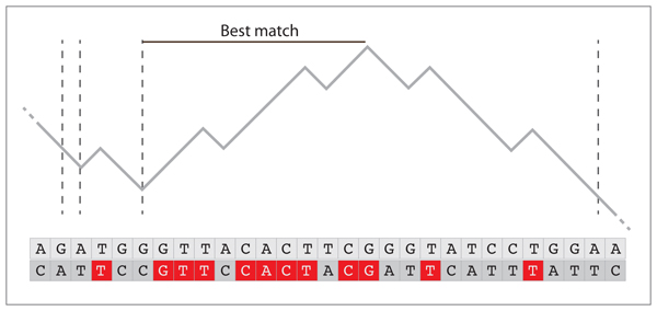
The figure above shows the correspondence between random walk and sequence alignment. The two DNA sequences correspond to database and query, respectively. In the case of simple sequence alignments, each match scores +1 (indicated by a red letter) and each mismatch scores -1. For random sequences, the alignment score is a simple random walk with a negative drift, in the case of DNA, the probability of a match is approximately $(1/4)$ because there are $(4)$ nucleotides. As shown in the figure above, the local maxima correspond to local best matches, and the extreme value of the maxima is the alignment score. Since the local maxima are IID, we need to find the asymptotic distribution of the extreme value of IID variables. The Fisher-Tippet-Gnedenko theorem applies, and since the distribution of the maximum has an exponential tail, the extreme value of those independent maxima has a Gumbel distribution.

The difficulty in the real proof is to identify the scaling and centering parameters of the asymptotic Gumbel distribution. In the case of protein alignments, an extra difficulty arises from the fact that the associated random walk is no longer binary. Since the possible steps are not integers neither integer multiples of each other, the random walk may have a null probability of returning to a previous state. This peculiarity does not change the asymptotic behavior of the walk, but it requires a more involved proof.

Anticipating the worst is something we need to do all the time, and in that respect extreme value theory deserves more attention. Once again, I blame p-values for causing a lot of confusion and giving a false feeling of control. Interpreted as “the probability of observing a more extreme result”, they prevent us from asking the right question... “what is the result, exactly?”

References

[1] Improved tools for biological sequence comparison. Pearson and Lipman, Proc Natl Acad Sci U S A. 1988 Apr;85(8):2444-8.
[2] Limit distribution of maximal segmental score among Markov-dependent partial sums. Karlin and Dembo, Adv Appl Prob. 1992 24:113-140.
[3] Extreme values in the GI/G/1 queue. Iglehart, The Annals of Mathematical Statistics. 1972 43(2):627-635.