In the first days of my PhD, I sincerely believed that there was a chance I would find a cure against cancer. As this possibility became more and more remote, and as it became obvious that my work would not mark a paradigm shift, I became envious of those few people who did change the face of science during their PhD. One of them is Andrey Kolmogorov, whose PhD work was nothing less than the modern theory of probability. His most famous result was the strong law of large numbers, which essentially says that random fluctuations become infinitesimal on average. Simply put, if you flip a fair coin a large number of times, the frequency that ‘tails’ turn up will be very close to the expected value 1/2.

The chaos of large numbers

Most fascinating about the strong law of large numbers is that it is a theorem, which means that it comes with hypotheses that do not always hold. There are cases that repeating a random experiment a very large number of times does not guarantee that you will get closer to the expected value — I wrote the gory detail on Cross Validated, for those interested. One case that the strong law of large numbers does not hold is that of distributions with infinite expectation.

The classical example of a random variable with infinite expectation is the Saint Petersburg lottery, that we already met in an earlier post. Briefly, you flip a coin until ‘heads’ turn up, doubling your gain every time ‘tails’ turn up. Your expected gain at every round of this simple gambling scheme is nothing less than infinite, which puts the Saint Petersburg lottery outside of the realm of the strong law of large numbers.

What happens if you decide to play the Saint Petersburg lottery anyway and record your average gain? It cannot be infinite because you always flip ‘heads’ at some point, so you always gain a finite amount of money every time. How can the expectation be infinite then? This is as disturbing as the famous Chuck Norris fact that

Chuck Norris counted to infinity — twice.

Well... to be accurate, it is only half as disturbing. But it has an explanation, which lies in the large deviations of the gambling process. The gains and losses will be small in general, until an epic gain is so high that whatever happened before becomes irrelevant in comparison.

The picture on the left shows the typical trajectory of a Saint-Petersburg lottery gambler with a fixed entry price of $5. The gambler first loses $40,000 but near round 35,000 wins more than $100,000 (a streak of 20 ‘tails’ in a row). Until round 35,000 the value of the average gain would seem to stabilize around a negative number, but it will suddenly shoot upwards and stay positive. If the process were allowed to continue, the average gain would keep going up, chaotically but inevitably. For this reason, there is no typical gain in this gambling scheme. The Saint-Petersburg lottery is driven by rare cataclysmic events, or by what Nassim Nicholas Taleb calls Black Swans.

The sloppy gene

The Saint Petersburg lottery is a toy example, it does not actually exist out there (to the possible exception of our banking system). So did Mother Nature produce such monsters at all? The answer is yes, and I learnt only recently that this is the case of diffusion.

At our scale, diffusion typically looks like the picture on the left. As you might expect, the purple liquid eventually fills the glass uniformly. No surprise. At the microscopic level though, the story is very different. The diffusion of a particle is best described by a type of random walk called Brownian motion. A particle diffusing on a line or on a plane will eventually reach every given point, however, the expected time until this happens is infinite. In a 3D space the situation is worse because the particle may never reach that given point.

For those interested in the mathematical detail, in the next technical section I derive the distribution of the return time in the case of the simple random walk using the Catalan numbers. Click on the Penrose triangle for more detail.

Let’s work the case of a drunk man who walks left or right randomly one step at a time. Just after he leaves the bar, the bartender realizes that the drunk man forgot his hat. He decides to put it back on his head next time he sees the drunk man in front of the bar. How long does he have to wait?

Leaving the bar, the drunk man takes one step to the left, say, which we will call the starting point. We are going to count the number of return paths to the bar. The most common way to do this is to use André's reflection method (the proof is on Wikipedia), but here I will use a recursive equation. Even though this approach is less intuitive, it highlights a more general mechanism, since several processes have the same combinatorics (the number of binary trees is such an example).

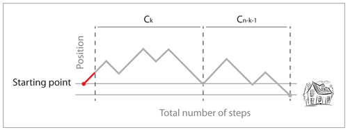
Let $(C_n)$ be the number of return paths to the bar with $(n)$ steps to the left (and thus $(n+1)$ steps to the right). $(C_0 = 1)$ because the only path from the starting point to the bar without any step to the left is the path that consists of one step to the right. For $(n > 0)$, observe that the drunk man must first step to the left, so that he is always one step left of the starting point (indicated by the red dash on the path), so every return path to the bar must first return to the starting point. The number of return paths to the starting point with $(k)$ steps to the left is $(C_k)$ by translation. Since such return paths contain $(k+1)$ steps to the left from the starting point, we can write the total number of return paths from the starting point to the bar as

$$C_n = \sum_{k=0}^{n-1} C_k C_{n-1-k}\; (n \geq 1).$$

In other words, a return path from the starting point to the bar consists of one step to the left, a return path to the starting point, and a return path to the bar. The solutions of this equation are the Catalan numbers

$$C_n = \frac{1}{n+1} {2n \choose n}.$$

The proof can be found on Wikipedia. If you are not convinced by the recurrence argument, you can encode the path of $(2n)$ steps by a sequence of brackets, opening for a step to the right, closing for a step to the left. A path returning to the starting point without crossing the bar contains as many opening and closing brackets, and never contains an unmatched closing bracket — corresponding to more steps to the left than steps to the right. The number of such sequences is known to be the Catalan number.

Since the total number of paths of $(2n)$ steps is $(4^n)$, the probability that the drunk man is at the starting point after $(2n)$ steps without ever crossing the bar is $(\frac{1}{n+1} {2n \choose n}\frac{1}{4^n})$, and the probability that he returns to the bar for the first time after $(2n+1)$ steps is half of that number (this is the probability of being at the starting point after $(2n)$ steps without crossing the bar and doing the next step to the left). In summary, the probability of first return after $(2n+1)$ steps when starting one step away from the bar is

$$P(2n+1) =\frac{1}{2} \frac{1}{n+1} {2n \choose n}\frac{1}{4^n}, n \geq 0.$$

This defines a proper probability distribution with infinite expected value. First we prove $(\sum_{n=0}^\infty P(2n+1) = 1)$. By developing $((1-x)^{-1/2})$ as an infinite series we obtain

$$\sum_{n=0}^\infty {2n \choose n} \frac{x^n}{4^n}.$$

Integrating both sides of the equality yields

$$C-2(1-x)^{1/2} = \sum_{n=0}^\infty \frac{1}{n+1} {2n \choose n} \frac{x^{n+1}}{4^n},$$

where $(C)$ is the integration constant. Setting $(x=0)$ yields $(C = 2)$, which for $(x = 1)$ gives the desired result. Next we prove that the expectation is infinite. That is

$$\frac{1}{2}\sum_{n=0}^\infty \frac{2n + 1}{n+1} {2n \choose n} \frac{1}{4^n} = \infty.$$

For this we use Stirling’s approximation which gives $({2n \choose n} \sim 4^n / \sqrt{\pi n})$. As $(n)$ goes to infinity, the general term of the series above is equivalent to $((\pi n)^{-1/2})$ so the series is divergent (series of general term proportional to $(n^{-\alpha})$ only converge for $(\alpha > 1)$). En passant we can also see that the distribution of the return time is asymptotic to a power law of exponent $(3/2)$, i.e. it is asymptotically proportional to $(n^{-3/2})$.

In the case of the one-dimensional Brownian motion, which is the continuous version of the simple random walk, the probability density of the waiting time of a particle starting at $(a)$ to reach $(0)$ is

$$\frac{|a|}{\sqrt{2\pi t^3}} e^{-a^2/2t}, t > 0.$$

The proof of this statement can be found for instance in this book. This probability density also has infinite expectation and is also asymptotically proportional to $(t^{-3/2})$.

The fact that diffusing molecules sometimes take extremely long before they reach their target is disastrous news for everything that is alive. As far as we know, gene expression is based on diffusion of transcription factors. These proteins need to diffuse to their target genes in order to activate or repress them, and if this is not done on time anything could go wrong. But the situation is far from desperate because cells use every trick to prevent those cataclysmic waiting times. In particular, biological molecules always diffuse within a finite volume, and there are usually more than just one diffusing molecule, which reduces the waiting time until any one of them hits the target. In addition, genomes are full of structures such as enhancers, which could act as transcription factor magnets in order to target them to the nearby genes. And of course, there is much more than this, as suggested by the animation below for instance.

The video features the scanning model of transcription factor diffusion, which is a cool idea to explain how transcription factors may not waste time in useless diffusion away from DNA. Unfortunately for this idea, DNA in a living cell does not look at all like the naked worms shown in the animation. At least in eukaryotes, DNA is wrapped around histones as I mention in my previous post, which makes the scanning of transcription factors practically impossible, since they would constantly bump into nucleosomes.

That said, the organization of the genome in the nucleus is still a mystery and perhaps the scanning model is at work in ways that we don’t yet understand. Theoretical arguments suggest that relying on simple diffusion would make gene regulation too sloppy and therefore that additional mechanisms are required to make the process efficient. But the truth is that we don’t know. Binding of transcription factors to DNA is still very poorly understood and reliable in vivo data is very scarce. Here is a real challenge for the years to come.